During one month, our Bourgogne-Franche-Comté region was in trouble: the music festival, called Franc-Tamponnage, for alternative, electronic and extreme kind was in progress. Our friends at Magna Vox planned dozens of concerts throughout the region.
For a specific set of concerts, we were in charge of creating a nice visual experience for visitors. It was the perfect opportunity for some creative coding! We were 3 coders on this project, Julien experimenting for the first time with openFrameworks, Tamsen playing around with one of his favorite toy: Processing and Aymeric making some good old Flash!
Here’s the recap by each of us :
Aymeric :
I worked on the poster designed by Le Tâche Papier and used a water ripples with AS3:

Tamsen :
I worked with Processing 3 to create a music controlled image distortion ‘visualizer’. Images were from a participating artist Pierre Berthier (black and white processed scans of sketches) so the base processing output was black on white, nothing fancy. It was then composited live and manipulated by a technician that had control over what and how things were projected, using Millumin.
Here’s an example :
The hope was to get live music to control how images changed and were distorted, the processing sketch was ready for such use, but due to technical and time constraints, a video of prerecorded processing output was sent through and looped, used as the technician saw fit during the concert.
Using the Processing library called minim by compartmental, a simple forward FFT is applied to the input audio. This allows us to get spectral data from the incoming signal, in short, we have a stream of values, each varying whether the sound has low, medium or high frequencies (the number of ‘divisions’ or bands you can extract from the signal can be determined in advance, we basically used 6).
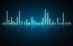
This is the most basic way to react to sound, and would be the same algorithm used to simply display a spectral visualization such as this one which we’ve all seen :
So you see, for each bands in the spectrum, we can play around with some parameters.
In this case, high frequencies would swap the image used, the image itself is displayed on a quad and that quad’s vertices are being moved in space as well as the uv’s themselves, there are also effects such as faked motion blur (made by not clearing the background of the buffer).
Here’s a simple patch to get started : 
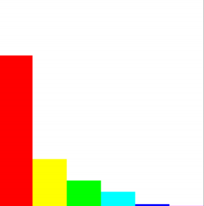
import ddf.minim.*; import ddf.minim.analysis.*; Minim minim; AudioInput input; FFT fft; int bands = 6; // number of 'bands' we wish to extract from the audio input float[] spectrum = new float[bands]; void setup() { size(600,600); minim = new Minim(this); //create minim input = minim.getLineIn(Minim.STEREO); //start line in (audio input) fft = new FFT(input.bufferSize(),input.sampleRate()); //create fft according to input fft.linAverages(bands); //setup for averages fft.window(FFT.GAUSS); //window algorithm background(255); smooth(4); colorMode(HSB); noStroke(); } float getFFT(int i) { float val = spectrum[i]; //Here, one could correct values, remap or scaled them based on index etc... return val; } void doSpectrum() { fft.forward(input.mix); for (int i = 0; i < bands; ++i) spectrum[i] = fft.getAvg(i); } void draw() { doSpectrum(); background(255); float d = (float)width/(float)bands; float hueDiv = 255.0/(float)bands; for(int i = 0;i < bands; i++) { color c = color(i*hueDiv,255,255); fill(c); float h = getFFT(i) * height; rect(i*d,height - h,d,h); } } void stop() { input.close(); minim.stop(); super.stop(); }This sample will just draw a histogram for the spectrum, You will also notice that as bands are higher in the frequency domain, values are smaller, one should (in getFFT for example) try to remap or scale values based on the band index to get more workable values, the code to do so is not included here for clarity and there could be many approaches.
Also to be clear, we’re calling bands averages of multiple bands – since we don’t want the full raw data the FFT would extract. Anyway this was enough for our use case. More complex sound analysis such as timbre analysis could be done with more audio oriented software such as Pure Data and the timbreID library which not only does FFT but finer analysis of the ‘nature’ of the sound let’s say . We almost were going to go this route but this would’ve involved wifi communication and some hardware we had no time to setup unfortunately.
Julien :
I was new in creative programming and I would use C++ to program procedural effects on Pierre Berthier pictures. So the famous and well documented OpenFrameworks was my choice for the development.
Cause the images are black and white, I preferred to put some colors and played with. In the constraint time, he develop 3 effects : Meta-balls, a liquid filling with particles emission, and a liquid spread effect.
Here’s an example on a holographic device during the festival :
The effects was not command by the music and we wanted to have control on the generation. A sequencer was develop to “randomize” the display with patterns (effects with different colors, background image, and other parameters). The patterns are stock in a json.
At the beginning, it was expected to generate the video at runtime in a embarked device, so we planned to use a Raspberry Pi 3. The Raspberry Pi is not a powerful computer, and programming effect on OpenFrameworks with OpenGL is not very efficient on high resolution (720p or 1080p). The Raspberry displayed effect between 25-32 FPS on 720p. So to boost performances, I wrote the most effects in shaders (meta-balls and liquid spreading).
Metaballs
The metaballs are simple implicit surface with only spheres. So the shader development wasn’t complicated. The tricky part was on the trails/fill effects.
FBO (FrameBuffer object) are use to create layer : one for rendering metaballs and one for the trails. On the trails layer, we render the metaballs with a alpha to do a accumulation effect.
During the effect, metaballs color change and is the same for the trails. The blend between the old color and the new color was hard to find. We leave the code of metaballs, maybe this will save your time.ofSetColor(255); int nbCircle = 10; float _metaballsCenter[nbCircle * 2]; float _metaballsSquareRadius[nbCircle]; _fbo.begin(); metaballsShader.begin(); metaballsShader.setUniform2fv("metaballsCenter", _metaballsCenter, _nbCircle); metaballsShader.setUniform1fv("metaballsSquareRadius", _metaballsSquareRadius, _nbCircle); metaballsShader.setUniform3f("inputColor", _currentColor.r*.0039215, _currentColor.g*.0039215, _currentColor.b*.0039215); _fbo.draw(0, 0); metaballsShader.end(); _fbo.end(); ofEnableAlphaBlending(); glBlendFuncSeparate(GL_SRC_ALPHA, GL_ONE_MINUS_SRC_ALPHA, GL_SRC_ALPHA, GL_ONE); ofSetColor(220, 220, 220, 20); _fbo2.begin(); _fbo.draw(0, 0); _fbo2.end(); ofEnableAlphaBlending(); ofSetColor(ofColor::white); _fbo2.draw(x, y); _fbo.draw(x, y);Liquid filling with particles
The effect combine 3 layers : particles, trails , and the “liquid”.
The particles are just circles with a basic physics (velocity + mass + gravitation).
The trails are similar to metaball’s trails. It’s a fbo with a semi-tranparent color apply every frame.
The liquid is a polygon with 3 border align to the screen limit and the last border design by a Perlin noise.Liquid spreading
The liquid spreading is a very simplified liquid physics. It’s based on a article of JGallant : http://www.jgallant.com/2d-liquid-simulator-with-cellular-automaton-in-unity/.
The effect is affected by a obstacle shape store in a image. The green channel is use, and the value of green mean the “height” of the obstacle at this pixel.
After on a other image, sources of color fluid are place. The liquid is store in pixel channel (r,g,b), so we can manage three different liquid at the same time.
At every frame, each pixels near pixels with liquid receive a fixed amount of liquid (color). In the process, the sources don’t lose liquid until the maximum level (255). So if a pixel is near of different color source, the color will be add in the pixel and blend the primaries color.
When a pixel is on an obstacle, we look the liquid level of the nearest pixel and the obstacle level. If the liquid level is higher than the obstacle, then the liquids color are added in the pixel.
Finally, for each primary color (rgb) a replacement color is set and the effect is done.


One thought on “Franc-Tamponnage and creative coding”